How to use Jupyter Notebooks in a Virtual Research Environment
Use the Platform's Software and Analysis areas to move from catalogue-driven exploration to notebook-based analysis in a Virtual Research Environment (VRE). This guide uses the Santorini area as the example.
The notebook-based approach keeps Platform services as the data source but moves the final part of the work into code, where you can change inputs, create custom outputs, and preserve the analysis state.
What this guide is for
Use notebook-based analysis when the standard Platform views are not enough and you need:
- programmatic access to the same services
- custom plots or custom map styling
- reproducible analysis steps
- a notebook state that can be saved, shared, or restored
If you need the Platform interface guide first, use How to explore the Platform interface. If you only need a prepared example workspace first, see Use Scientific Examples as a prepared starting point.
Find the notebook in the Software catalogue
We will start in Software, because that is where the reusable notebook entries appear. Open the Software area from the left navigation, look for Analyze earthquakes, permanent displacement and geology in the catalogue panel, and use the card title and category to confirm that you have the right resource.
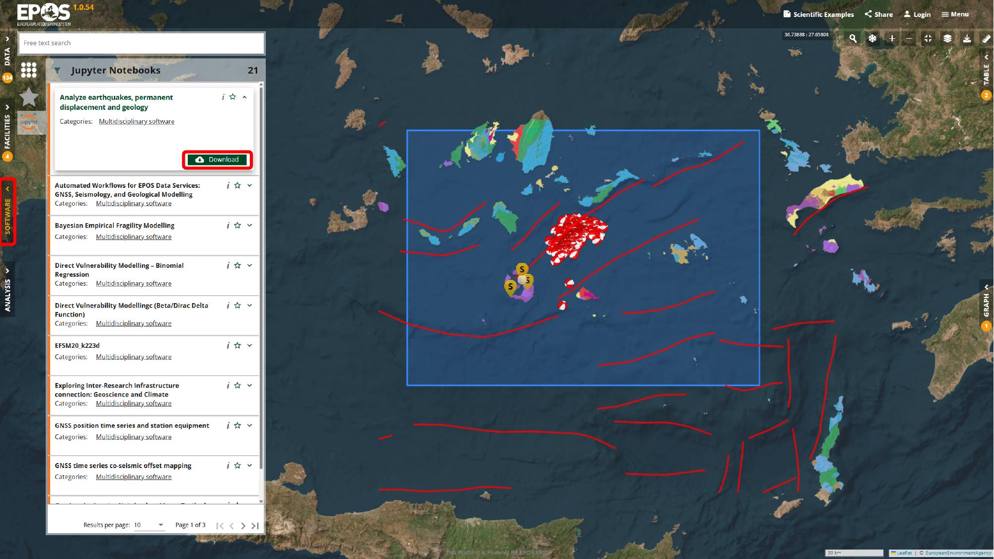
At this stage we are still in catalogue mode. The main thing we are doing is identifying the notebook resource that can either be downloaded for local use or attached to a VRE environment.
Decide between local download and VRE analysis
From that notebook entry, you usually have two valid paths forward:
- use Download if you want the
.ipynbfile for local use outside the Platform - continue with the VRE path if you want to run the notebook inside a Platform-connected analysis environment
For the rest of this guide, we will follow the VRE path. That is the more integrated option when you want to keep working close to the Platform services rather than exporting the notebook and running it elsewhere.
Open the Analysis area and sign in
The next step is a shift in context: we move from browsing notebook resources to managing an environment where the notebook can run. Open Analysis from the left navigation, use Login in the environment panel, and sign in with one of the identity providers available in your deployment.
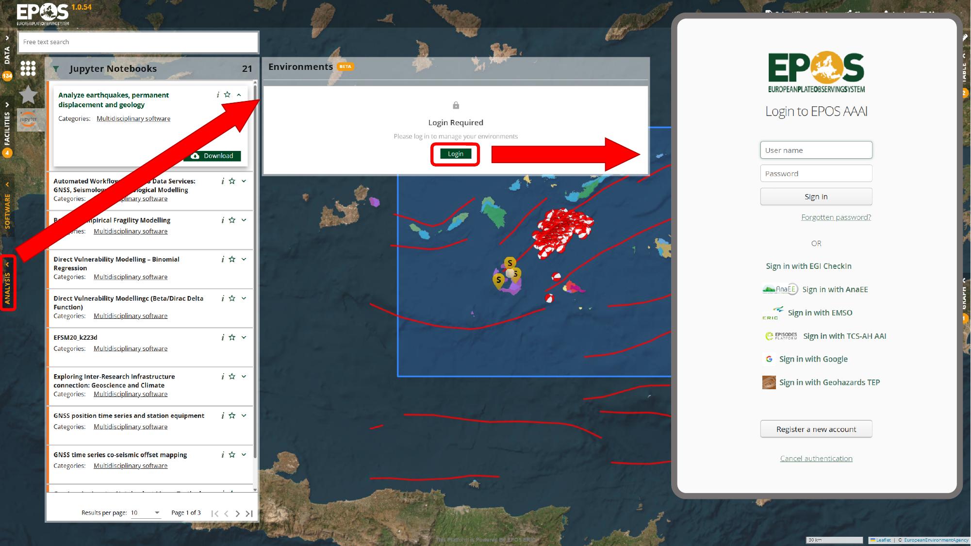
Once you are signed in, the Environments panel becomes available. That is where we create or reopen the notebook environment that will host the resource.
Create a notebook environment
If a suitable environment does not already exist, create one now. In the Environments panel, use Create Environment, call it Santorini, choose Jupyter Notebook as the environment type, pick the provider available in the deployment, and then confirm with the Create button in the dialog.
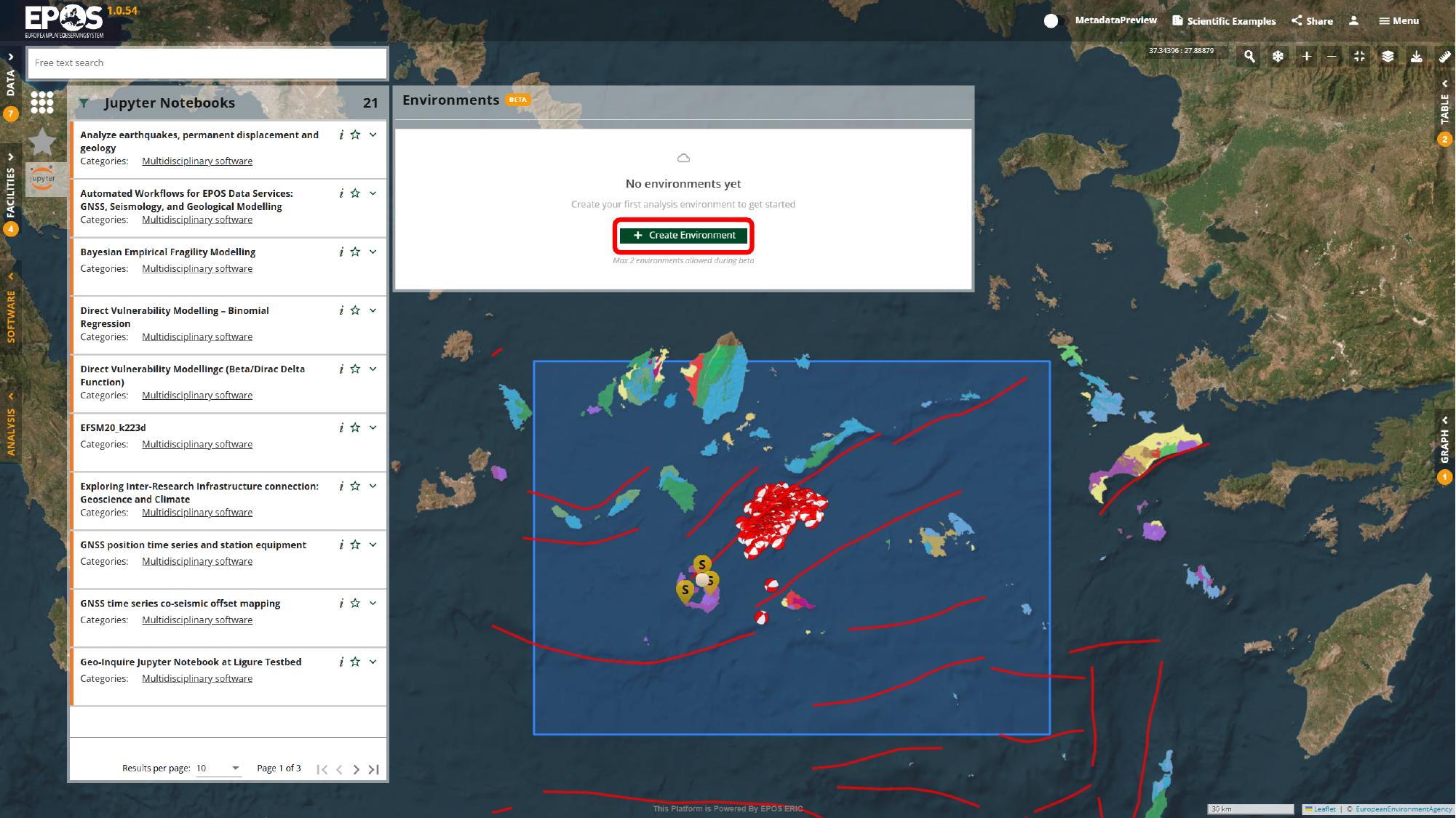
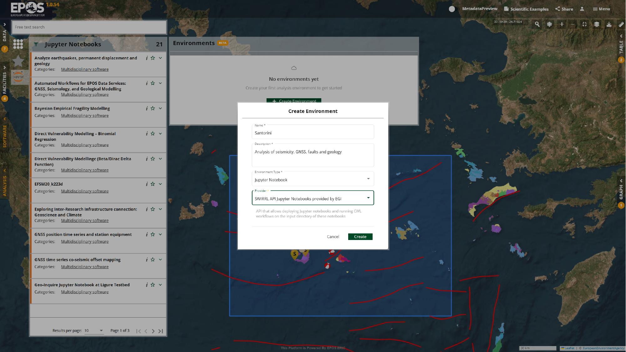
The names of the providers and some configuration options may differ between deployments, but the logic stays the same: sign in, create the environment, and prepare a place where the notebook can run.
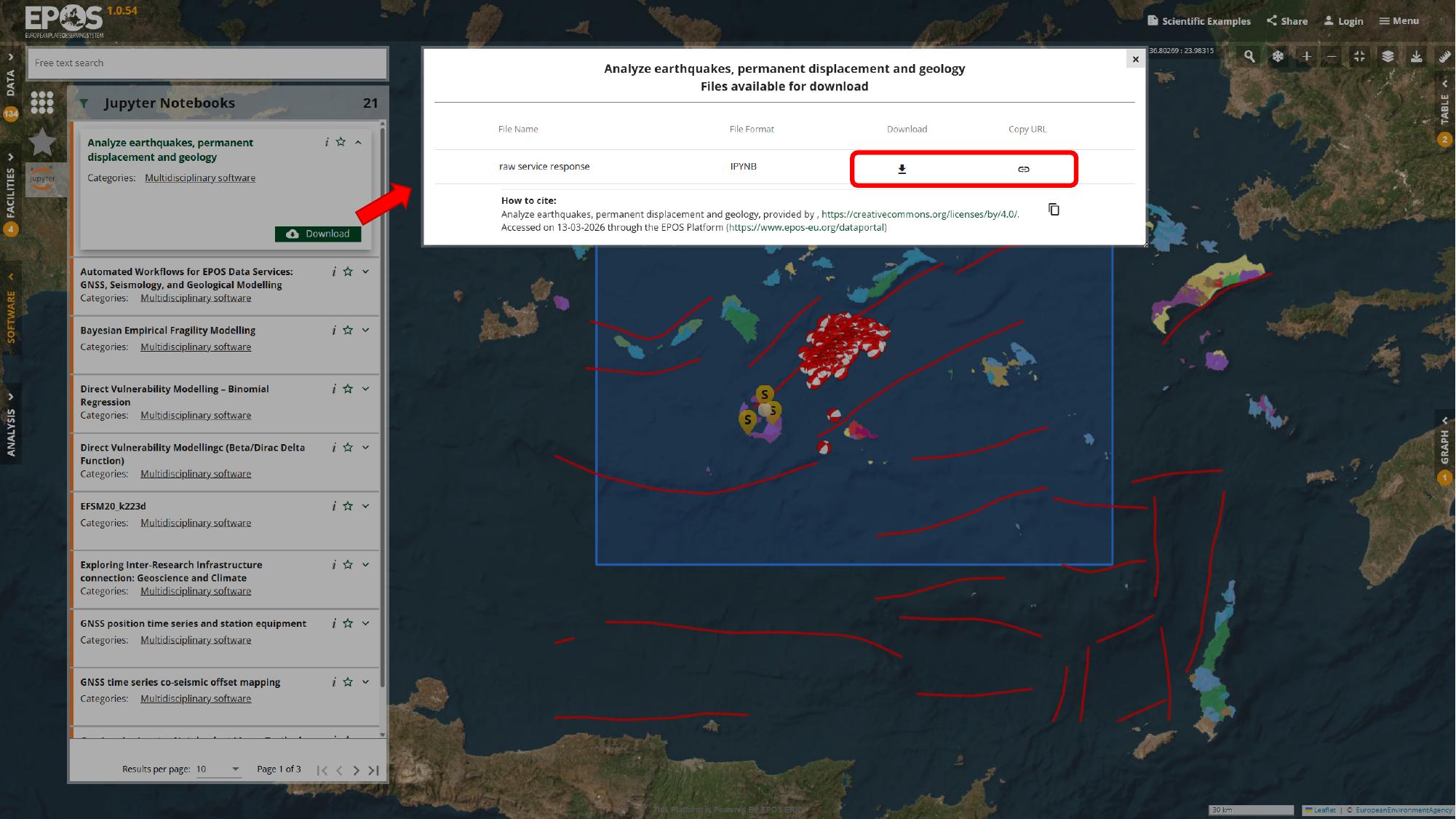
Add the notebook resource to the environment
Now we can connect the notebook resource to that environment. Return to the notebook entry in Software, open the file actions for the notebook (the Download button), and use Add to environment for the .ipynb file from that dialog.
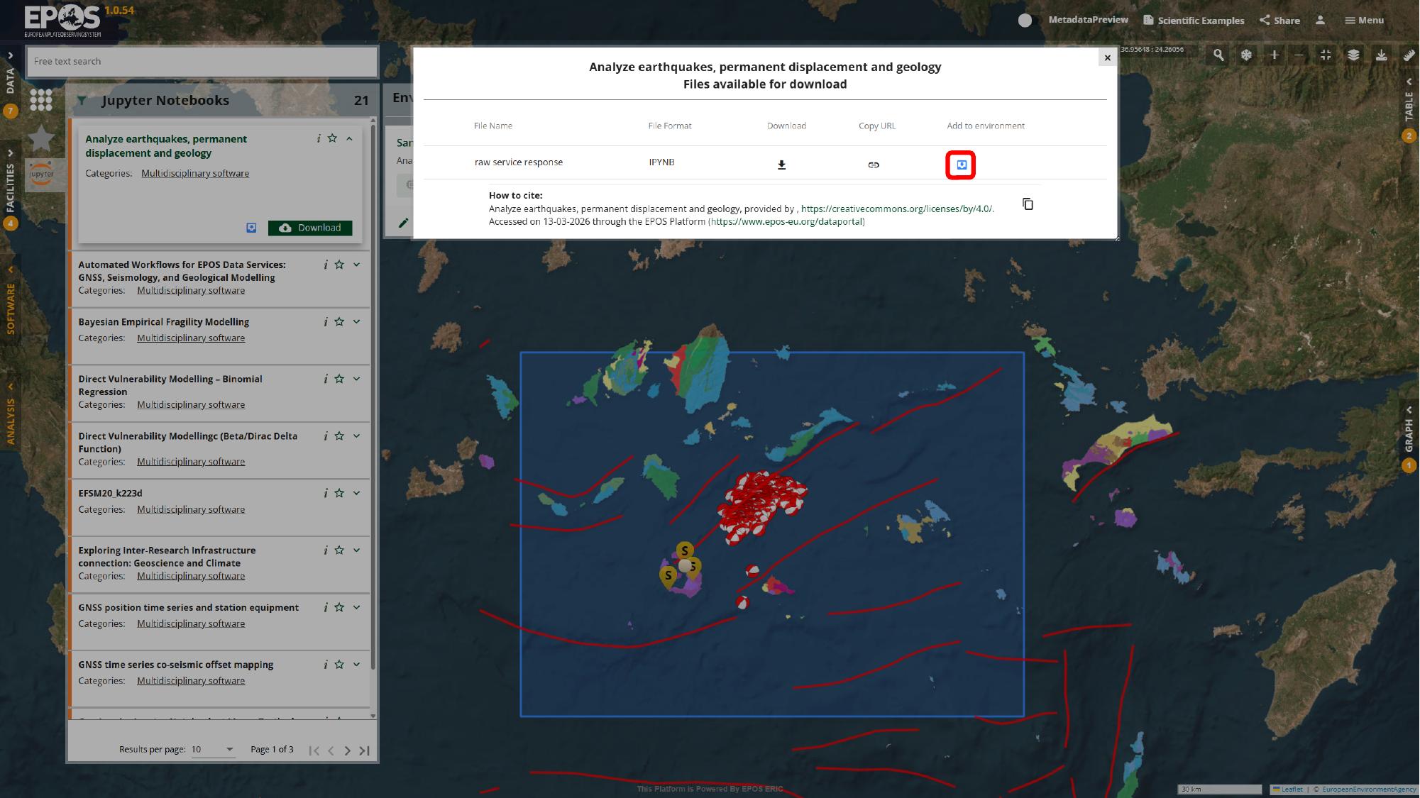
At that point the notebook is no longer just an item in the catalogue. It becomes a resource in the selected environment, which is what lets the VRE open it in a working analysis session.
Start the environment and open JupyterLab
After the notebook is attached, back in the Analysis tab, the environment usually moves through a short creation phase before it becomes ready to open. Watching that status change is useful because it tells you when the work is about to leave the Platform interface and continue inside JupyterLab.
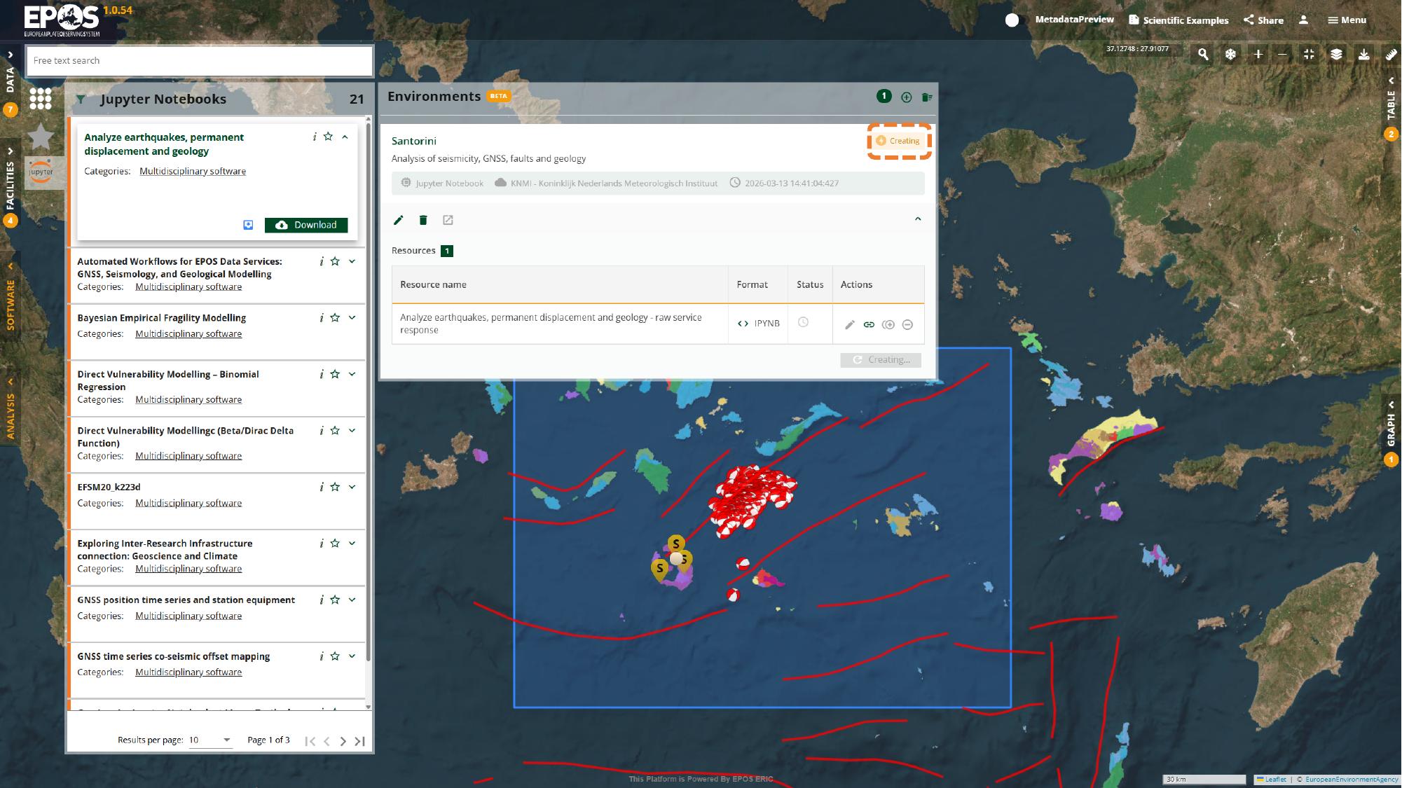
Once the environment reaches Ready, use its launch action in the environment card to open it.
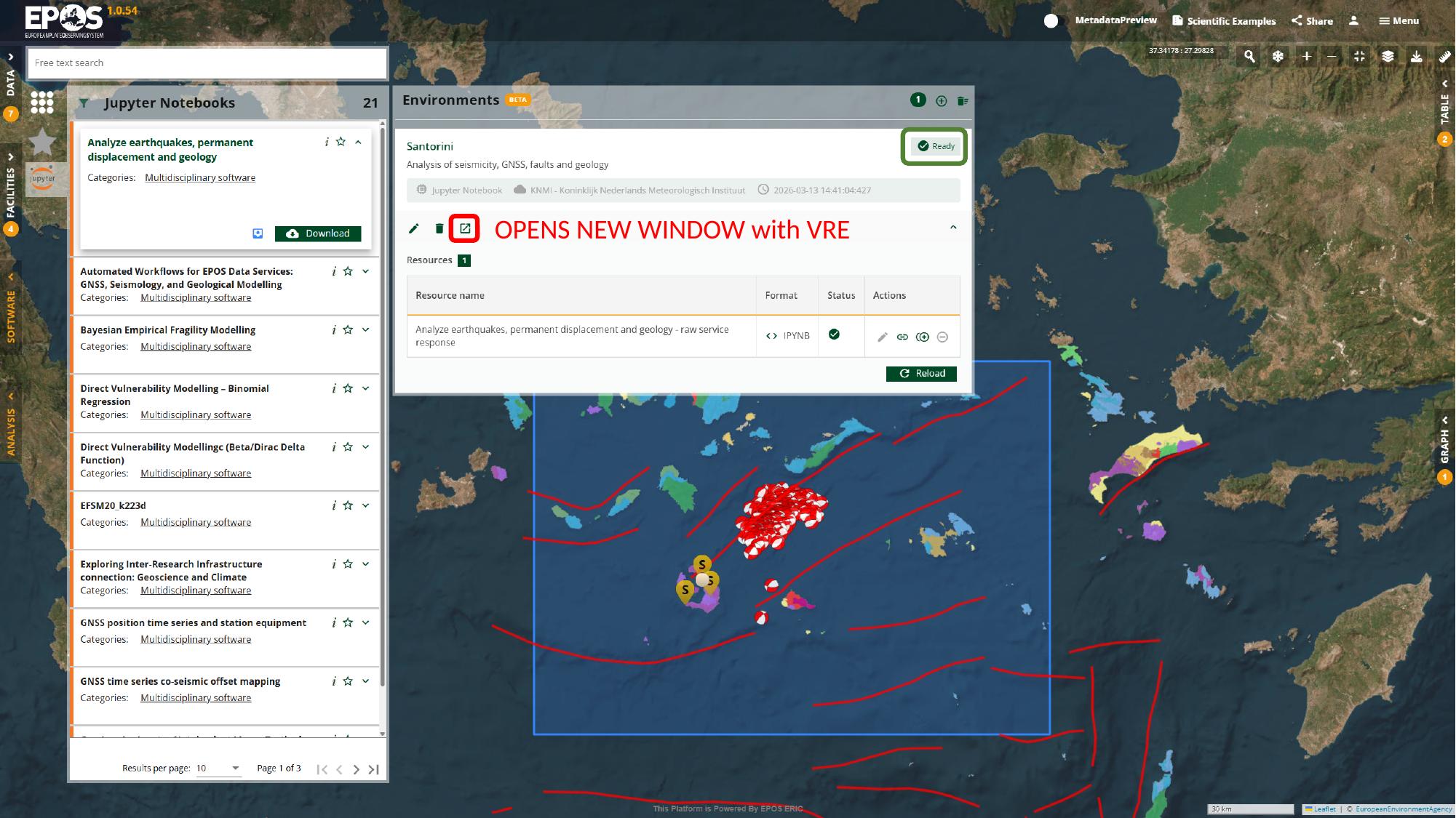
This is the handover point between the Platform UI and the notebook workspace. From here on, the interaction happens in JupyterLab rather than in the catalogue panels.
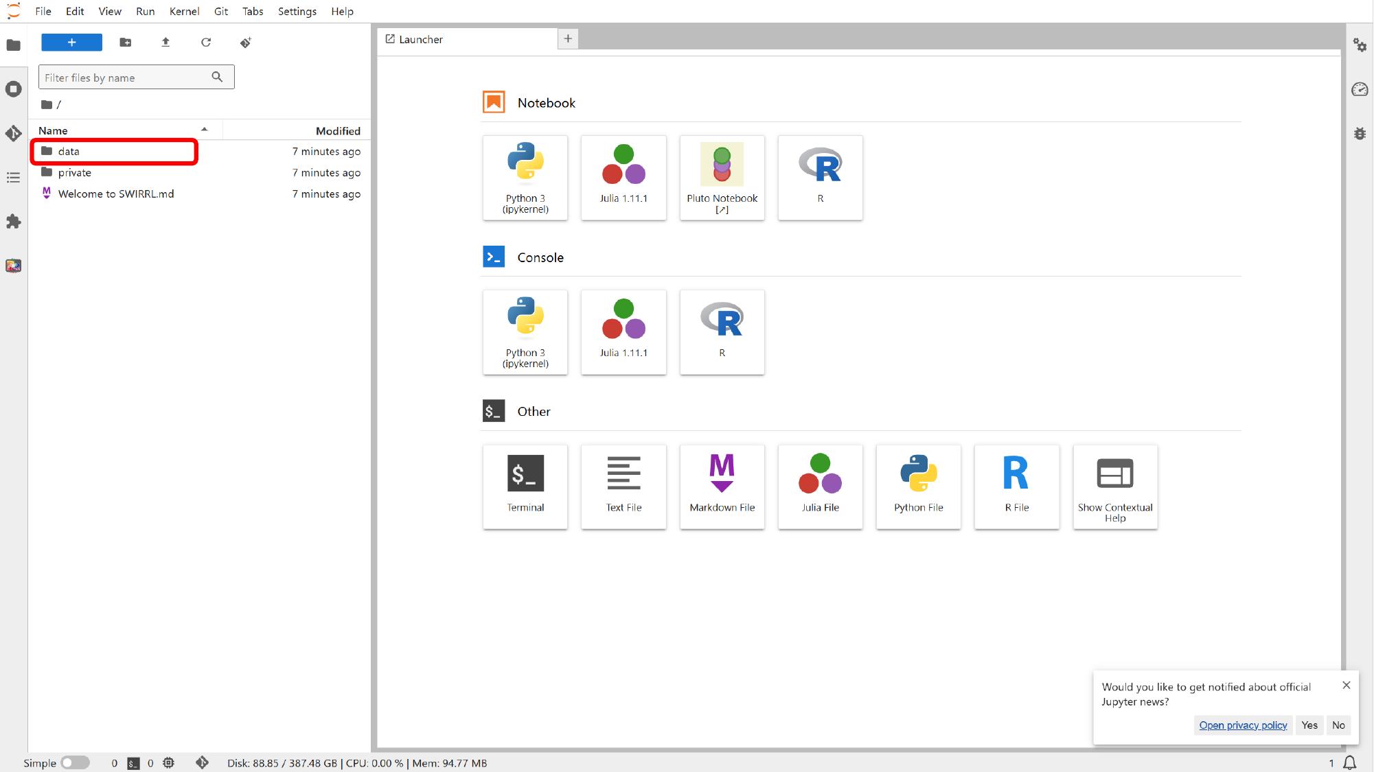
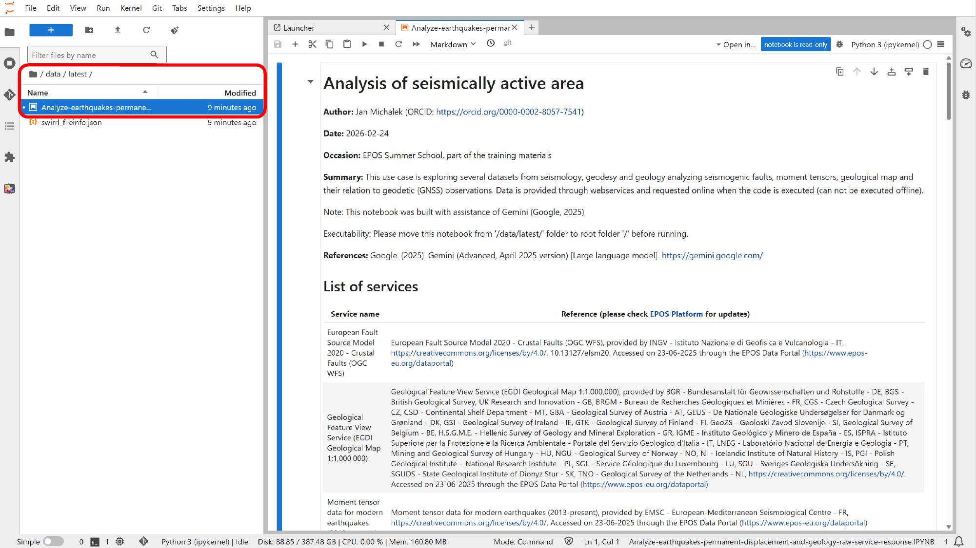
Open the notebook and review its structure
Inside JupyterLab, use the file browser on the left to look for the notebook resource under the data area. Some deployments place it directly in data/, while others use a data/latest/ subfolder or a similar resource directory.
Once the notebook is open, it is worth scanning the first section before changing anything. In this example, the opening cells explain the purpose of the notebook, list the services it uses, and show how the notebook is organized.
Edit the main input cell
Near the start of the notebook, the main user-controlled inputs are grouped together. That is usually the right place to adapt the notebook for another area or another time window.
For this example, click into that input cell and focus on the bounding box, the start time, and the end time.
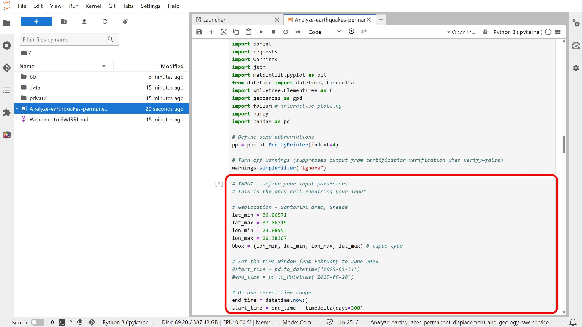
After those values change, rerun the dependent cells so the maps and plots reflect the updated parameters. This is one of the clearest differences from the standard Platform interface: here the notebook is still connected to Platform services, but the logic is now explicit and editable in code.
Run the notebook and inspect the outputs
Once the inputs are set, we can let the notebook produce outputs that go beyond the built-in Platform views.
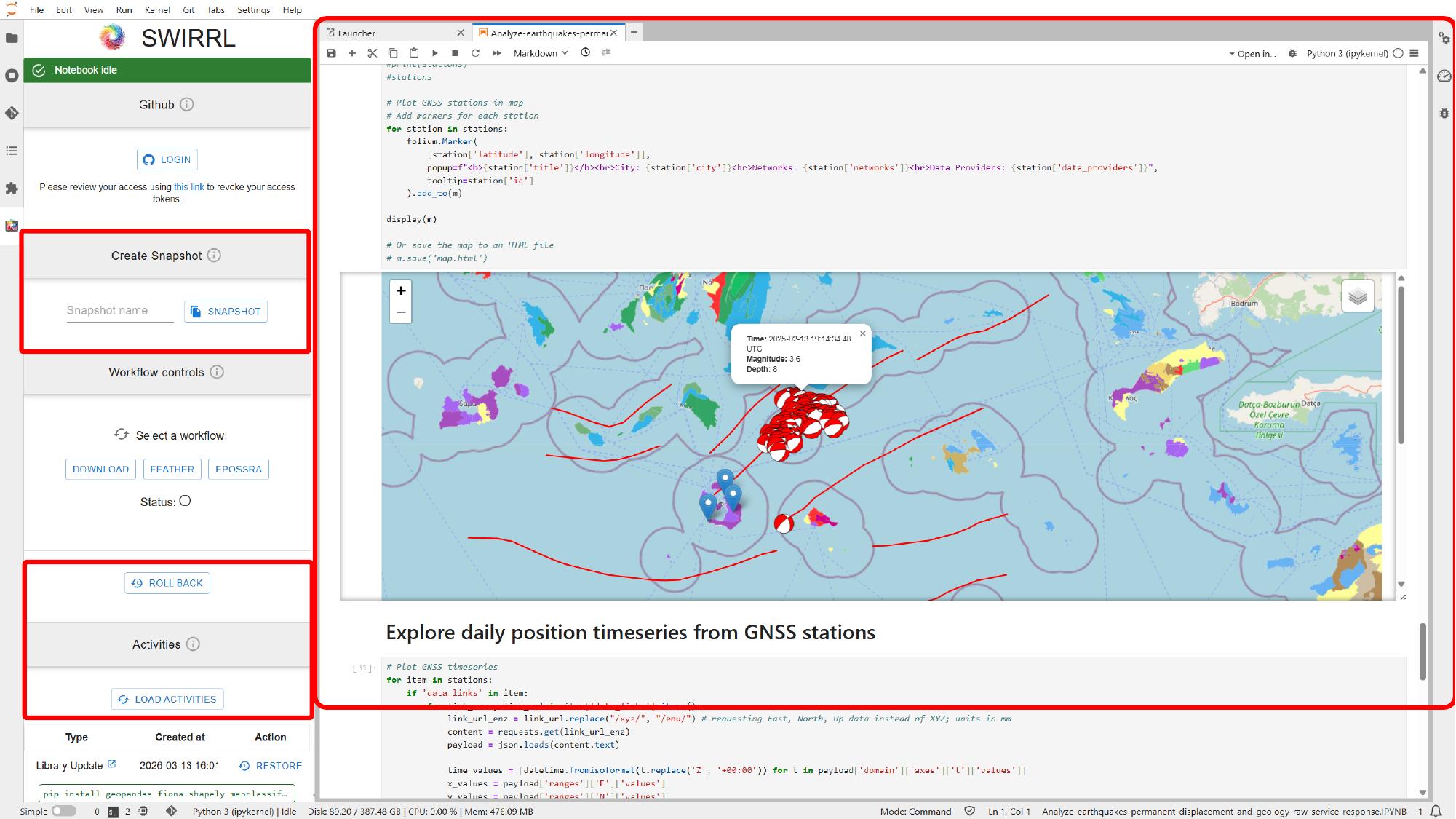
Inspect the interactive map output
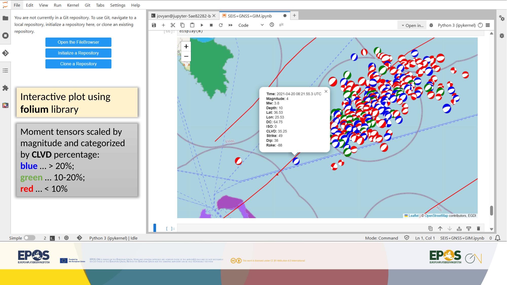
When the cells that fetch the data and render the map finish running, using the notebook run controls or the normal Jupyter cell execution flow, the notebook can show an interactive map directly inside JupyterLab.
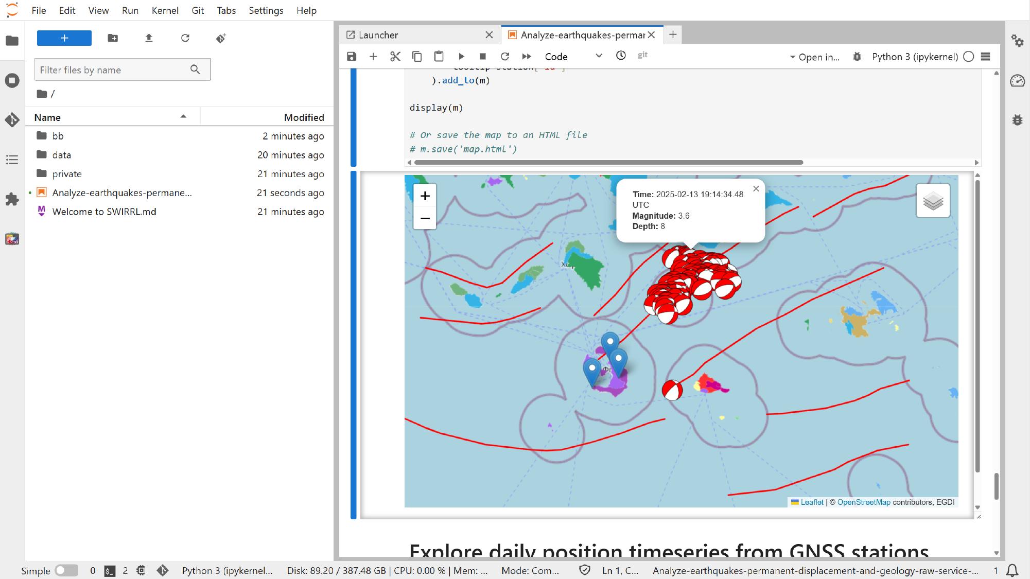
This is useful because the notebook is no longer limited to the default Platform styling. In this example, one of the visualizations color-codes moment tensors by CLVD percentage. The scientific meaning is notebook-specific, but the broader lesson is simple: notebooks let us reshape the same Platform data into more tailored views.
Inspect the additional plots
As the remaining analysis cells run, using the same notebook execution controls, the notebook can also generate plots that would not normally appear in the standard Platform interface, such as cumulative seismic moment plots or GNSS time-series plots assembled directly in code.
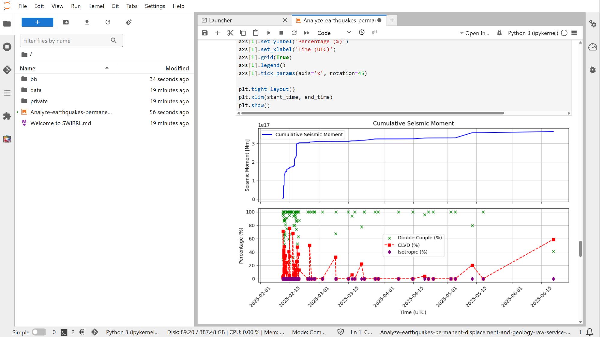
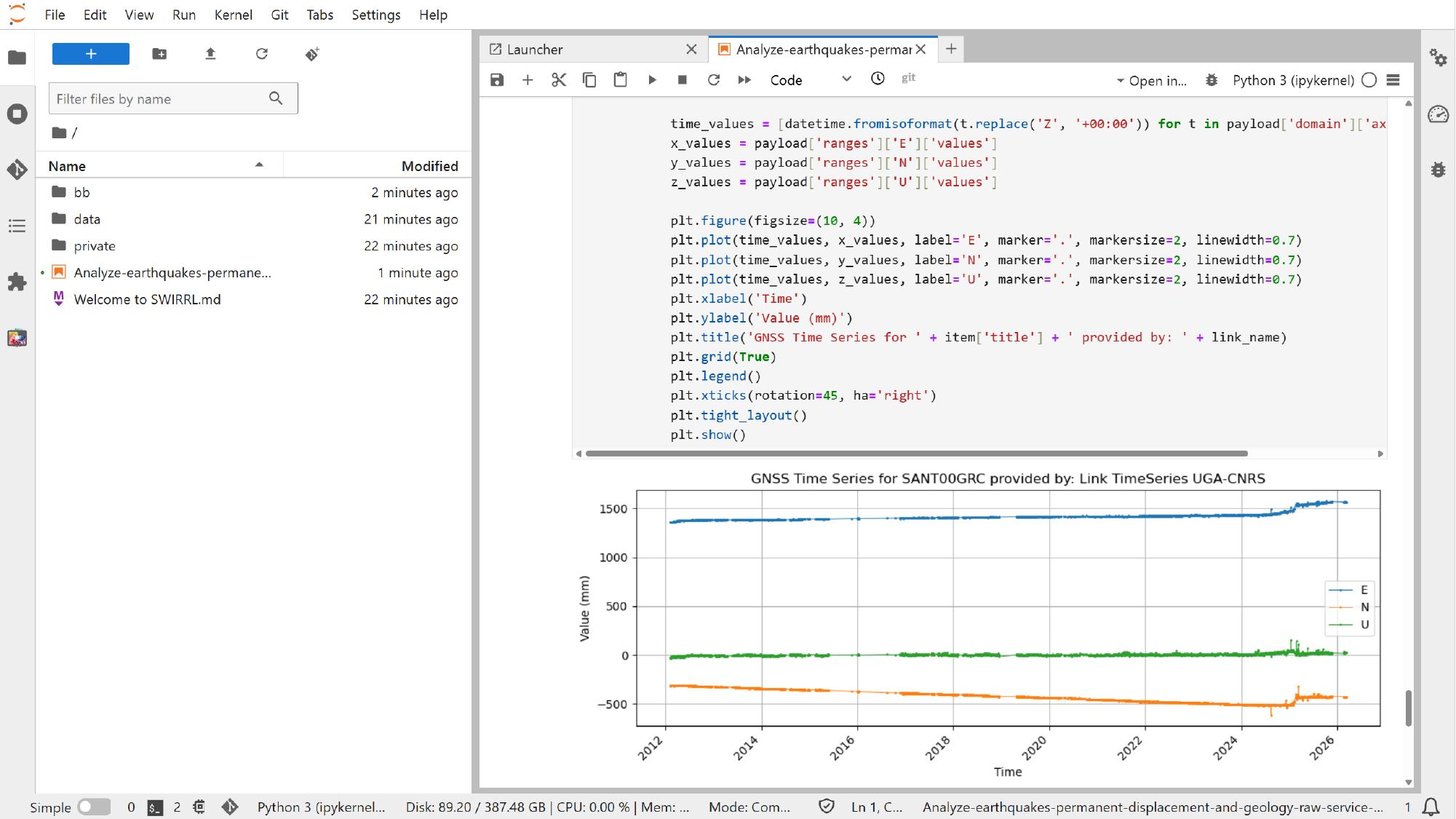
This is where notebook-based analysis shows its main value: the services still come from the Platform, but the final analysis becomes more flexible, reproducible, and easier to adapt.
Save, share, and recover the notebook state
The management features shown in this section are not part of standard JupyterLab alone. In deployments like this one, the VRE is typically provided through the open source SWIRRL VRE, which adds Jupyter-based environments together with extra controls for provenance tracking, snapshots, GitHub integration, rollback, and activity history through its SWIRRL extension.
The exact set of tools available in your environment still depends on the deployed image and configuration. If you need more detail on those SWIRRL-specific features, use the upstream SWIRRL VRE documentation as the main reference.
If snapshot or GitHub integration is available, use those controls in the VRE side panel to save the current state or publish the work outside the VRE.
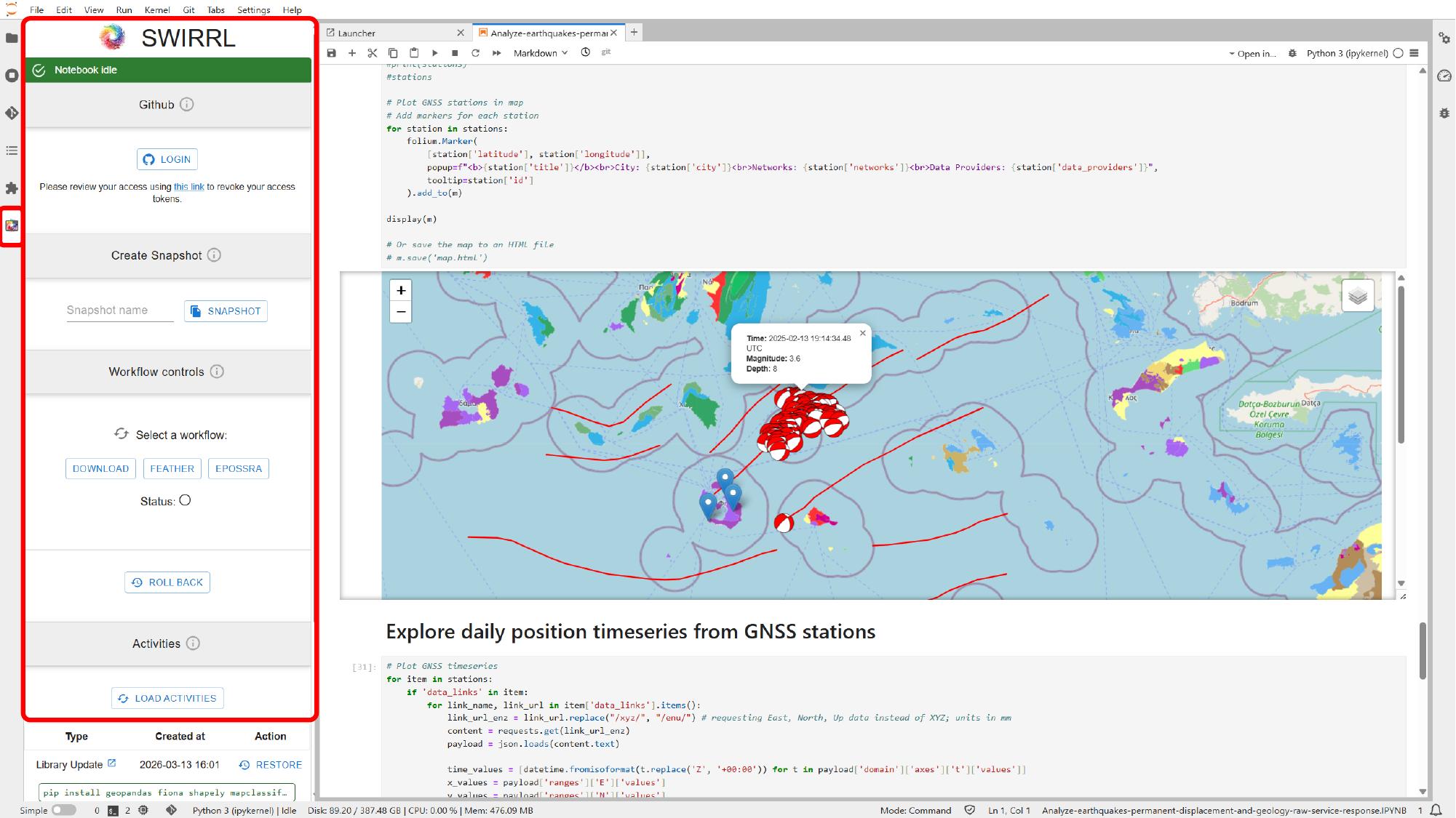
If rollback or activity history is available, use those controls in the same VRE side panel to return to an earlier working state after a failed change or an experiment you do not want to keep.
At this point, we have moved from the Platform interface into a notebook environment, adjusted the main inputs, and used the same Platform services to produce maps and plots in code. Once this approach feels familiar, you can reuse it for other areas, time windows, and notebook resources, while keeping the analysis easier to adapt, save, and reproduce.